用 layout() 进行图形组合
文章目录
这个内容是看完 MSG 之后的补课。
图形组合其实以往用过很多种了,base R 里的 par(mfrow = c(), mfcol = c()), ggplot2 里的 facet_grid() 和 facet_wrap() ,还有非常好用的 cowplot 的 plot_grid()。但是前者自定义性差,只能做很简单任务;后者则是 ggplot2 系统,并且是将同一个数据的作图根据指定变量来分割。而 layout() 则兼具了语法简洁和作图灵活的特点。cowplot 很不错,我们后面介绍⚑。
注意,文档里提醒:
These functions are totally incompatible with the other mechanisms for arranging plots on a device: ‘par(mfrow)’, ‘par(mfcol)’ and ‘split.screen’.
即 layout() 和 par(mfrow), par(mfcol) 以及 split.screen() 都是完全不相容的。split.screen() 也是一个很灵活的可以分割作图的方法,后面有空再写⚑。
先来一个最简单的 Quick Start:
nf <- layout(matrix(c(1, 1, 1,
                      2, 3, 4,
                      2, 3, 4), nr = 3, byrow = TRUE))
hist(rnorm(25), col = "VioletRed")
hist(rnorm(25), col = "VioletRed")
hist(rnorm(25), col = "VioletRed")
hist(rnorm(25), col = "VioletRed")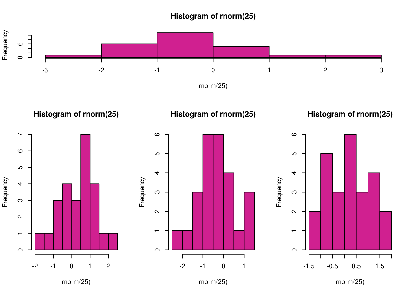
可以得到这样一幅图:
layout() 语法不了解的话初看起来完全看不懂,但是其实学习了之后就会发现既简单又灵活。它最主要的是接受一个 matrix 来定义图形布局。比如在上面的例子里我们定义了一个 3 x 3 的矩阵,矩阵数字只有 1/2/3/4。这个数字就是编号,表示整幅图会有 4 个小图。现在再把这个 3 x 3 矩阵想象成一个图片,整个图片被分成 3 行 3 列一共 9 个小格子,然后要画的 4 个小图怎么排布到 9 个小格子呢?看矩阵!矩阵里相应位置是几就放第几幅小图。有的位置有重复的话就表示一幅小图占用了不止一个小格子的位置。所以回过头再看上面的例子,我们定义的 3 行 3 列的布局里,第一行都是 1,表示第一幅图会占据这个图片第一行的位置,依此类推,下面的第二、三行都是一个小图占用两行的高度和 1/3 列的宽度。这样这个图片的布局就一目了然了。
layout() 也支持查看布局:
nf <- layout(matrix(c(1, 1, 1,
                      2, 3, 4,
                      2, 3, 4), nr = 3, byrow = TRUE))
layout.show(nf)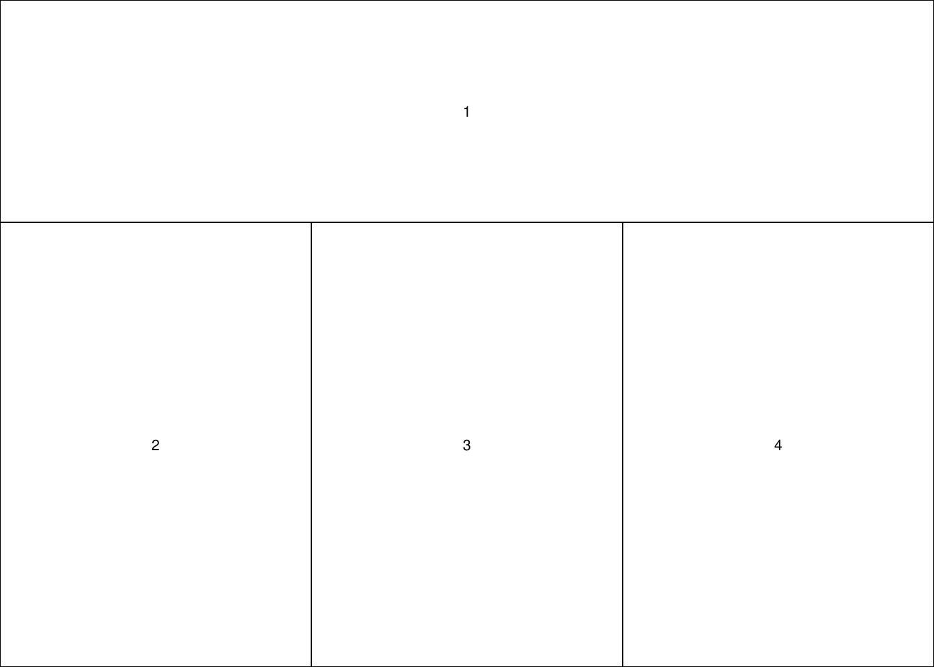
另外 layout() 还可以用 widths 和 heights 参数自己设置各个部分的高度的宽度。比如我们可以重现上面的布局:
nf <- layout(matrix(c(1, 1, 1,
                      2, 3, 4), nr = 2, byrow = TRUE),
             widths = c(1, 1, 1), heights = c(1, 2))
layout.show(nf)
再来看看文档里的例子:
set.seed(100)
n <- 100
x <- pmin(3, pmax(-3, stats::rnorm(n)))
y <- pmin(3, pmax(-3, stats::rnorm(n)))
xhist <- hist(x, breaks = seq(-3, 3, 0.5), plot = FALSE)
yhist <- hist(y, breaks = seq(-3, 3, 0.5), plot = FALSE)
top <- max(c(xhist$counts, yhist$counts))
xrange <- c(-3, 3)
yrange <- c(-3, 3)
nf <- layout(matrix(c(2, 0, 1, 3),
                    2, 2, byrow = TRUE),
             c(3, 1), c(1, 3), TRUE)
layout.show(nf)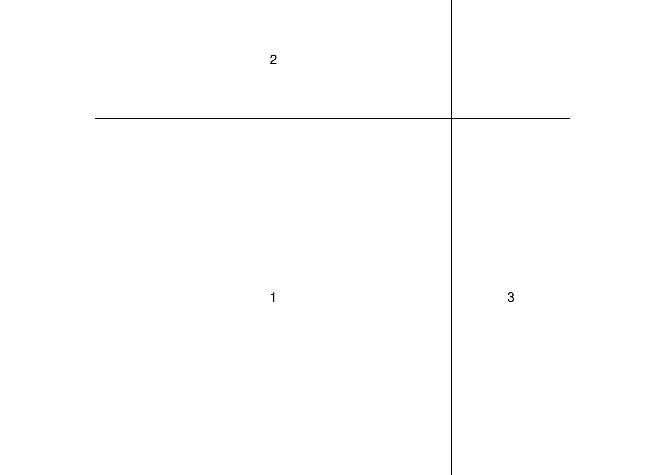
par(mar = c(3, 3, 1, 1))
plot(x, y,
     xlim = xrange, ylim = yrange,
     xlab = "", ylab = "")
par(mar = c(0, 3, 1, 1))
barplot(xhist$counts,
        axes = FALSE,
        ylim = c(0, top),
        space = 0)
par(mar = c(3, 0, 1, 1))
barplot(yhist$counts, axes = FALSE,
        xlim = c(0, top), space = 0,
        horiz = TRUE)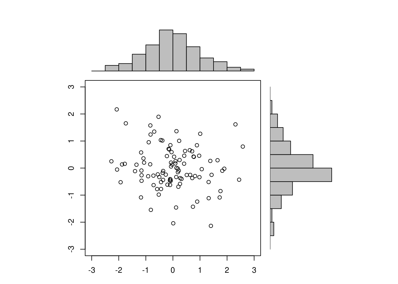
这个例子里一个很有意思的设置是矩阵里的 0 用做占位。
最后作为 One More Thing(虽然我也不是果粉),来看看 par(fig) 的一个例子:
par(fig = c(0, 0.8, 0, 0.8), new = TRUE)
plot(mtcars$wt, mtcars$mpg,
     xlab = "Car Weight",
     ylab = "Miles Per Gallon")
par(fig = c(0, 0.8, 0.55, 1), new = TRUE)
boxplot(mtcars$wt, horizontal = TRUE, axes = FALSE)
par(fig = c(0.65, 1, 0, 0.8), new = TRUE)
boxplot(mtcars$mpg, axes = FALSE)
mtext("Enhanced Scatterplot",
      side = 3, outer = TRUE, line = -2)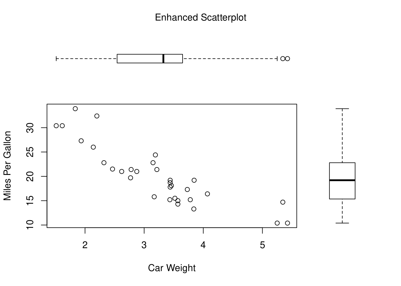
fig 参数接受一个形如 c(x1, x2, y1, y2) 的 NDC (normalized device coordinates) 参数,比如上面的例子里 fig = c(0, 0.8, 0, 0.8) 表示这幅图的位置是 X 轴 c(0, 0.8) 和 Y 轴 c(0, 0.8),即分别规定了宽度和高度及其对应的位置。
好吧,写短一点,就这样吧。PEACE…
参考:
文章作者 Jackie
上次更新 2020-05-15 (71e2f3e)