All models are wrong, but some are useful. – George Box
最近处理数据发现统计学知识太不够用了,以前上的统计学基本只知道 t 检验、方差分析、卡方检验加上简单的回归和相关、生存分析。对于 Logistic 回归知道的基本上就是怎么做的 logit 变换、回归系数 $ \beta$ 和 OR 的联系、怎么解释的问题。具体的怎么做生存分析、 Logistic 回归完全不知道。但是呢,实际做数据分析发现二者其实简直不要太常见。所以,只能自学了。
在网上随意搜找到一个很不错的材料,介绍 Bayesian Model Averaging 法的 R 包 BMA 用来做模型选择:Model Selection in Linear Regression ,似乎是 USTC 某位老师的教案。试着重复了一下里面的结果,大致还行。记录并且简单翻译一下。
讲义一共有 3 个例子,前两个都是模拟数据,所以其实我们是知道真实模型的,这样也可以方便的评价得到的结果是否准确;第 3 个也是最后一个模型是真实数据(低体重儿数据集)。
Example 1: Large number of covariates, null model is true
第一个例子使用模拟数据,数据有 30 个自变量 x 1000 个观测,但所有自变量都与因变量无关,即 null model 为真。我们通过这个例子比较 AIC 和 BIC 在真实模型很小(或简单)的时候的表现。
首先我们随机生成 15 个二分类变量 x1 ~ x15,每个变量都有不同比例的 0/1 。
 1
 2
 3
 4
 5
 6
 7
 8
 9
10
11
12
13
14
15
16
17
18
19
20
|
library("BMA")

rates <- round(seq(.1, .9, length.out=15), 2)

set.seed(1234)
x1 <- rbinom(1000, 1, rates[1])
x2 <- rbinom(1000, 1, rates[2])
x3 <- rbinom(1000, 1, rates[3])
x4 <- rbinom(1000, 1, rates[4])
x5 <- rbinom(1000, 1, rates[5])
x6 <- rbinom(1000, 1, rates[6])
x7 <- rbinom(1000, 1, rates[7])
x8 <- rbinom(1000, 1, rates[8])
x9 <- rbinom(1000, 1, rates[9])
x10 <- rbinom(1000, 1, rates[10])
x11 <- rbinom(1000, 1, rates[11])
x12 <- rbinom(1000, 1, rates[12])
x13 <- rbinom(1000, 1, rates[13])
x14 <- rbinom(1000, 1, rates[14])
x15 <- rbinom(1000, 1, rates[15])
|
然后是 15 个随机的标准正态分布(均数为 0, 标准差为 1)的连续型变量 x16 ~ x30:
 1
 2
 3
 4
 5
 6
 7
 8
 9
10
11
12
13
14
|
x16 <- rnorm(1000)
x17 <- rnorm(1000)
x18 <- rnorm(1000)
x19 <- rnorm(1000)
x20 <- rnorm(1000)
x21 <- rnorm(1000)
x22 <- rnorm(1000)
x23 <- rnorm(1000)
x24 <- rnorm(1000)
x25 <- rnorm(1000)
x26 <- rnorm(1000)
x27 <- rnorm(1000)
x28 <- rnorm(1000)
x29 <- rnorm(1000)
|
以及因变量 y 为随机的 0/1 各占一半:
1
|
y <- rbinom(1000, 1, 0.5)
|
搞定了,现在就直接把数据合起来就行了:
 1
 2
 3
 4
 5
 6
 7
 8
 9
10
11
12
13
14
15
16
17
18
19
20
21
22
23
24
25
26
27
28
29
30
|
example1.dat <- data.frame(y, x1, x2, x3, x4, x5, x6, x7, x8, x9, x10,
                           x11, x12, x13, x14, x15, x16, x17, x18, x19, x20,
                           x21, x22, x23, x24, x25, x26, x27, x28, x29, x30)
names(example1.dat)
#  [1] "y"   "x1"  "x2"  "x3"  "x4"  "x5"  "x6"  "x7"  "x8"  "x9"  "x10" "x11" "x12"
# [14] "x13" "x14" "x15" "x16" "x17" "x18" "x19" "x20" "x21" "x22" "x23" "x24" "x25"
# [27] "x26" "x27" "x28" "x29" "x30"

head(example1.dat)
#   y x1 x2 x3 x4 x5 x6 x7 x8 x9 x10 x11 x12 x13 x14 x15     x16      x17      x18
# 1 1  0  0  0  1  0  0  0  0  1   1   1   1   1   1   1 -0.9153  0.18906  0.56731
# 2 1  0  0  0  0  1  0  0  1  1   1   1   1   1   1   1 -1.0493  1.05886 -1.17934
# 3 1  0  0  0  0  0  1  1  0  1   1   1   1   1   1   1 -0.1702  1.50806  0.17732
# 4 0  0  0  0  0  0  1  0  1  0   1   0   1   0   1   1 -0.9573 -0.02743  0.09387
# 5 1  0  0  0  0  0  0  1  1  1   0   1   1   1   1   1 -0.4233  0.90592  0.37780
# 6 0  0  0  0  0  1  1  1  1  0   0   1   1   0   1   1 -0.2224  1.25207  0.67417
#        x19      x20     x21     x22     x23     x24     x25     x26      x27
# 1  0.05605  0.04794 -0.7579 -0.8885 -3.0130  0.2757 -0.9264 -1.0521 -1.95695
# 2 -0.01062  0.68691 -2.0385  0.5615 -0.6655  0.4172  0.2077 -0.7733 -0.28024
# 3 -0.20261  0.04087  0.3963 -0.0361  1.0232  0.3932  0.3591  0.9562 -1.42667
# 4 -1.01466 -0.12076  0.5976 -1.1644 -1.4597 -1.6077 -1.1000 -0.5926 -0.78517
# 5  0.37537  1.11574 -0.3029  1.0581 -0.4303  0.8402 -0.5158  0.8154 -0.02503
# 6  0.80737 -0.24688 -0.8890  0.8670 -0.6931  0.1868  0.7015 -1.5567  0.54382
#       x28     x29      x30
# 1  0.1325 -0.7575 -0.30341
# 2  0.2063  2.0019 -1.07430
# 3 -1.3397 -2.2955  0.40950
# 4 -1.2289 -0.7128 -0.48585
# 5  0.8574 -0.2103 -1.42814
# 6  1.0331  0.4169  0.03321
|
下面就可以用 BMA 包的 bic.glm 开始分析了。再次提醒一下,这个数据里 null model 为真!
命令形式为:
1
2
3
4
5
|
bic.glm(f, data, glm.family, wt = rep(1, nrow(data)),
    strict = FALSE, prior.param = c(rep(0.5, ncol(x))), OR = 20,
    maxCol = 30, OR.fix = 2, nbest = 150, dispersion = NULL,
    factor.type = TRUE, factor.prior.adjust = FALSE,
    occam.window = TRUE, ...)
|
其实好多参数我是根本不懂的,具体的还得看 ?bic.glm,这也是我要补习统计的地方…
行吧,先直接跑吧:
1
2
3
4
5
|
fml <- as.formula(paste0("y ~",
                         paste(names(example1.dat[, -y]), collapse = ' + ')))
output1 <- bic.glm(fml, glm.family = "binomial",
                   data = example1.dat, maxCol = 31)
summary(output1)
|
输出实在太长,放图片吧:
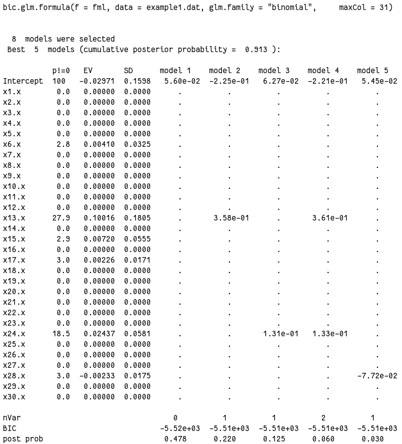
从结果可以看到,从选出的 8 个模型里最佳的 5 个模型中,null model 确实排在第一位。后验概率 0.478。而排在后面的几个模型后验概率都要小得多。
我们再看看其他的输出,8 个模型的后验概率和包含的变量:
1
2
3
4
5
|
output1$postprob
# [1] 0.47782 0.21993 0.12541 0.05956 0.03011 0.02977 0.02920 0.02821

output1$label
# [1] "NULL"        "x13.x"       "x24.x"       "x13.x,x24.x" "x28.x"       "x17.x"       "x15.x"       "x6.x"
|
对于所有变量来说,每个变量应该包含在模型里的可能性:
1
2
3
4
5
|
output1$probne0
 #  x1   x2   x3   x4   x5   x6   x7   x8   x9  x10  x11  x12  x13  x14  x15  x16
 # 0.0  0.0  0.0  0.0  0.0  2.8  0.0  0.0  0.0  0.0  0.0  0.0 27.9  0.0  2.9  0.0
 # x17  x18  x19  x20  x21  x22  x23  x24  x25  x26  x27  x28  x29  x30
 # 3.0  0.0  0.0  0.0  0.0  0.0  0.0 18.5  0.0  0.0  0.0  3.0  0.0  0.0
|
x13 竟然神奇的达到了 27.9%,x24 也有 18.5,而原文这里最高的也只有 15.1%。
 1
 2
 3
 4
 5
 6
 7
 8
 9
10
11
12
13
14
15
16
17
18
19
20
21
22
23
24
25
26
27
28
29
30
31
32
33
34
35
36
37
38
39
40
41
42
43
44
45
46
47
48
49
50
51
52
53
54
55
56
57
58
59
60
61
62
63
64
65
66
67
68
69
70
|
xtabs(~y + x13, data = example1.dat)
#    x13
# y     0   1
#   0 119 367
#   1  95 419
chisq.test(xtabs(~y + x13))
#
# 	Pearson's Chi-squared test with Yates' continuity correction
#
# data:  xtabs(~y + x13)
# X-squared = 5, df = 1, p-value = 0.03


t.test(x24 ~ y, data = example1.dat, var.equal = TRUE)
#
# 	Two Sample t-test
#
# data:  x24 by y
# t = -2.1, df = 1000, p-value = 0.04
# alternative hypothesis: true difference in means is not equal to 0
# 95 percent confidence interval:
#  -0.252496 -0.005981
# sample estimates:
# mean in group 0 mean in group 1
#        -0.11523         0.01401

fit.2 <- glm(y ~ x13 + x24, data = example1.dat, family = binomial())
# summary(fit.2)
# Call:
# glm(formula = y ~ x13 + x24, family = binomial(), data = example1.dat)
#
# Deviance Residuals:
#    Min      1Q  Median      3Q     Max
#  -1.37   -1.20    1.03    1.14    1.38
#
# Coefficients:
#             Estimate Std. Error z value Pr(>|z|)
# (Intercept)  -0.2209     0.1379   -1.60    0.109
# x13           0.3607     0.1554    2.32    0.020 *
# x24           0.1326     0.0642    2.07    0.039 *
# ---
# Signif. codes:  0 ‘***’ 0.001 ‘**’ 0.01 ‘*’ 0.05 ‘.’ 0.1 ‘ ’ 1
#
# (Dispersion parameter for binomial family taken to be 1)
#
#     Null deviance: 1385.5  on 999  degrees of freedom
# Residual deviance: 1375.9  on 997  degrees of freedom
# AIC: 1382
#
# Number of Fisher Scoring iterations: 3

1 - pchisq(1385.5-1375.9, 999 - 997, lower.tail = FALSE)
# [1] 0.99

anova(fit.2, test = 'Chisq')
# Analysis of Deviance Table
#
# Model: binomial, link: logit
#
# Response: y
#
# Terms added sequentially (first to last)
#
#
#      Df Deviance Resid. Df Resid. Dev Pr(>Chi)
# NULL                   999       1386
# x13   1     5.36       998       1380    0.021 *
# x24   1     4.30       997       1376    0.038 *
# ---
# Signif. codes:  0 ‘***’ 0.001 ‘**’ 0.01 ‘*’ 0.05 ‘.’ 0.1 ‘ ’ 1
|
这就尴尬了,只含有 x13 和 x24 的模型怎么分析来看都是成立的,只能说是天意吧 😂
贝叶松模型平均值和标准差(我也不知道具体的意义🤦):
 1
 2
 3
 4
 5
 6
 7
 8
 9
10
11
12
13
14
15
16
|
output1$postmean
# (Intercept)          x1          x2          x3          x4          x5          x6
#   -0.029711    0.000000    0.000000    0.000000    0.000000    0.000000    0.004100
#          x7          x8          x9         x10         x11         x12         x13
#    0.000000    0.000000    0.000000    0.000000    0.000000    0.000000    0.100163
#         x14         x15         x16         x17         x18         x19         x20
#    0.000000    0.007204    0.000000    0.002262    0.000000    0.000000    0.000000
#         x21         x22         x23         x24         x25         x26         x27
#    0.000000    0.000000    0.000000    0.024373    0.000000    0.000000    0.000000
#         x28         x29         x30
#   -0.002326    0.000000    0.000000
output1$postsd
#  [1] 0.15977 0.00000 0.00000 0.00000 0.00000 0.00000 0.03251 0.00000 0.00000 0.00000
# [11] 0.00000 0.00000 0.00000 0.18053 0.00000 0.05550 0.00000 0.01714 0.00000 0.00000
# [21] 0.00000 0.00000 0.00000 0.00000 0.05811 0.00000 0.00000 0.00000 0.01746 0.00000
# [31] 0.00000
|
以及所有模型的估计值及其标准误:
 1
 2
 3
 4
 5
 6
 7
 8
 9
10
11
12
13
14
15
16
17
18
19
20
21
22
23
24
25
26
27
28
29
30
31
32
33
34
35
36
37
38
39
40
41
42
43
44
45
46
47
48
|
output1$mle
#      (Intercept) x1 x2 x3 x4 x5     x6 x7 x8 x9 x10 x11 x12    x13 x14    x15 x16
# [1,]   5.601e-02  0  0  0  0  0 0.0000  0  0  0   0   0   0 0.0000   0 0.0000   0
# [2,]  -2.252e-01  0  0  0  0  0 0.0000  0  0  0   0   0   0 0.3578   0 0.0000   0
# [3,]   6.266e-02  0  0  0  0  0 0.0000  0  0  0   0   0   0 0.0000   0 0.0000   0
# [4,]  -2.209e-01  0  0  0  0  0 0.0000  0  0  0   0   0   0 0.3607   0 0.0000   0
# [5,]   5.451e-02  0  0  0  0  0 0.0000  0  0  0   0   0   0 0.0000   0 0.0000   0
# [6,]   5.358e-02  0  0  0  0  0 0.0000  0  0  0   0   0   0 0.0000   0 0.0000   0
# [7,]  -1.671e-01  0  0  0  0  0 0.0000  0  0  0   0   0   0 0.0000   0 0.2467   0
# [8,]   1.350e-16  0  0  0  0  0 0.1453  0  0  0   0   0   0 0.0000   0 0.0000   0
#        x17 x18 x19 x20 x21 x22 x23    x24 x25 x26 x27      x28 x29 x30
# [1,] 0.000   0   0   0   0   0   0 0.0000   0   0   0  0.00000   0   0
# [2,] 0.000   0   0   0   0   0   0 0.0000   0   0   0  0.00000   0   0
# [3,] 0.000   0   0   0   0   0   0 0.1314   0   0   0  0.00000   0   0
# [4,] 0.000   0   0   0   0   0   0 0.1326   0   0   0  0.00000   0   0
# [5,] 0.000   0   0   0   0   0   0 0.0000   0   0   0 -0.07724   0   0
# [6,] 0.076   0   0   0   0   0   0 0.0000   0   0   0  0.00000   0   0
# [7,] 0.000   0   0   0   0   0   0 0.0000   0   0   0  0.00000   0   0
# [8,] 0.000

output1$se
#         [,1] [,2] [,3] [,4] [,5] [,6]   [,7] [,8] [,9] [,10] [,11] [,12] [,13]
# [1,] 0.06327    0    0    0    0    0 0.0000    0    0     0     0     0     0
# [2,] 0.13758    0    0    0    0    0 0.0000    0    0     0     0     0     0
# [3,] 0.06349    0    0    0    0    0 0.0000    0    0     0     0     0     0
# [4,] 0.13792    0    0    0    0    0 0.0000    0    0     0     0     0     0
# [5,] 0.06333    0    0    0    0    0 0.0000    0    0     0     0     0     0
# [6,] 0.06335    0    0    0    0    0 0.0000    0    0     0     0     0     0
# [7,] 0.20484    0    0    0    0    0 0.0000    0    0     0     0     0     0
# [8,] 0.08071    0    0    0    0    0 0.1301    0    0     0     0     0     0
#       [,14] [,15]  [,16] [,17]   [,18] [,19] [,20] [,21] [,22] [,23] [,24]   [,25]
# [1,] 0.0000     0 0.0000     0 0.00000     0     0     0     0     0     0 0.00000
# [2,] 0.1551     0 0.0000     0 0.00000     0     0     0     0     0     0 0.00000
# [3,] 0.0000     0 0.0000     0 0.00000     0     0     0     0     0     0 0.06404
# [4,] 0.1554     0 0.0000     0 0.00000     0     0     0     0     0     0 0.06416
# [5,] 0.0000     0 0.0000     0 0.00000     0     0     0     0     0     0 0.00000
# [6,] 0.0000     0 0.0000     0 0.06533     0     0     0     0     0     0 0.00000
# [7,] 0.0000     0 0.2154     0 0.00000     0     0     0     0     0     0 0.00000
# [8,] 0.0000     0 0.0000     0 0.00000     0     0     0     0     0     0 0.00000
#      [,26] [,27] [,28]   [,29] [,30] [,31]
# [1,]     0     0     0 0.00000     0     0
# [2,]     0     0     0 0.00000     0     0
# [3,]     0     0     0 0.00000     0     0
# [4,]     0     0     0 0.00000     0     0
# [5,]     0     0     0 0.06584     0     0
# [6,]     0     0     0 0.00000     0     0
# [7,]     0     0     0 0.00000     0     0
# [8,]     0     0     0 0.00000     0     0
|
可以通过比较这个表格里模型间估计值的不同来鉴定有没有混杂因素和共线性之类的。
最后来看看模型的可视化 imageplot.bma(output1):
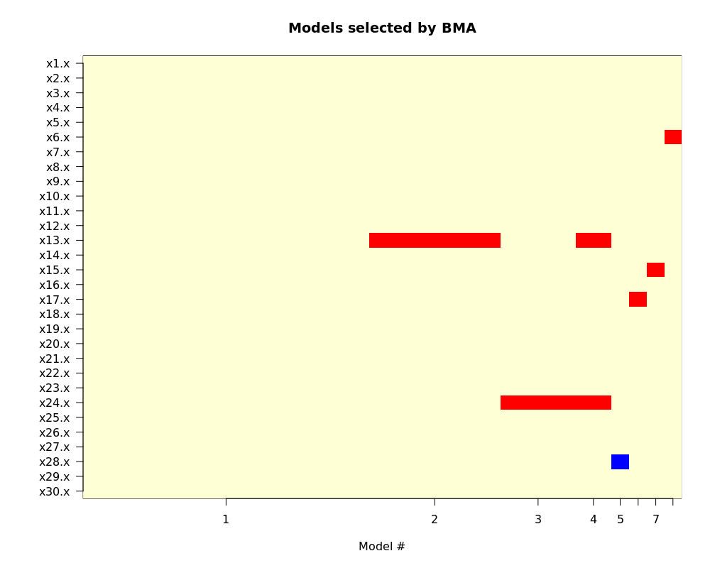
图中红色表示系数为正,蓝色为负。
不管怎么样,BIC 总体表现还行吧,至少最优模型确实是 null 嘛。下面再看 AIC 的情况:
 1
 2
 3
 4
 5
 6
 7
 8
 9
10
11
12
13
14
15
16
17
18
19
20
21
22
23
24
25
26
27
28
29
30
31
32
33
34
35
36
37
38
39
40
41
42
43
44
45
46
47
48
49
50
51
52
53
|
output1.aic <- glm(fml, data = example1.dat, family = binomial(link = 'logit'))
summary(output1.aic)

# Call:
# glm(formula = fml, family = binomial(link = "logit"), data = example1.dat)
#
# Deviance Residuals:
#    Min      1Q  Median      3Q     Max
#  -1.52   -1.19    0.94    1.13    1.49
#
# Coefficients:
#              Estimate Std. Error z value Pr(>|z|)
# (Intercept) -0.444427   0.373099   -1.19    0.234
# x1          -0.000796   0.200521    0.00    0.997
# x2          -0.060975   0.188152   -0.32    0.746
# x3          -0.005271   0.156950   -0.03    0.973
# x4           0.141855   0.147306    0.96    0.336
# x5          -0.103934   0.137558   -0.76    0.450
# x6           0.136568   0.132909    1.03    0.304
# x7           0.046675   0.130489    0.36    0.721
# x8          -0.054424   0.129178   -0.42    0.674
# x9           0.036636   0.130852    0.28    0.779
# x10          0.073951   0.133445    0.55    0.579
# x11         -0.026379   0.136114   -0.19    0.846
# x12         -0.038997   0.146629   -0.27    0.790
# x13          0.372992   0.157420    2.37    0.018 *
# x14         -0.118615   0.175837   -0.67    0.500
# x15          0.283099   0.219810    1.29    0.198
# x16         -0.019169   0.065982   -0.29    0.771
# x17          0.076281   0.066948    1.14    0.255
# x18          0.044459   0.065549    0.68    0.498
# x19          0.013658   0.065620    0.21    0.835
# x20          0.002741   0.063851    0.04    0.966
# x21          0.010957   0.065941    0.17    0.868
# x22         -0.030705   0.065102   -0.47    0.637
# x23          0.040860   0.064653    0.63    0.527
# x24          0.128399   0.065797    1.95    0.051 .
# x25         -0.019262   0.062303   -0.31    0.757
# x26          0.050657   0.062493    0.81    0.418
# x27         -0.012711   0.064273   -0.20    0.843
# x28         -0.078285   0.067635   -1.16    0.247
# x29          0.008709   0.066532    0.13    0.896
# x30         -0.019270   0.064948   -0.30    0.767
# ---
# Signif. codes:  0 ‘***’ 0.001 ‘**’ 0.01 ‘*’ 0.05 ‘.’ 0.1 ‘ ’ 1
#
# (Dispersion parameter for binomial family taken to be 1)
#
#     Null deviance: 1385.5  on 999  degrees of freedom
# Residual deviance: 1365.8  on 969  degrees of freedom
# AIC: 1428
#
# Number of Fisher Scoring iterations: 4
|
可以看到 x13 仍然很显著,x24 交界性 p 值。step 一下:
 1
 2
 3
 4
 5
 6
 7
 8
 9
10
11
12
13
14
15
16
17
18
19
20
21
22
23
24
25
26
|
step.aic1 <- step(output1.aic)
summary(step.aic1)
#
# Call:
# glm(formula = y ~ x13 + x24, family = binomial(link = "logit"),
#     data = example1.dat)
#
# Deviance Residuals:
#    Min      1Q  Median      3Q     Max
#  -1.37   -1.20    1.03    1.14    1.38
#
# Coefficients:
#             Estimate Std. Error z value Pr(>|z|)
# (Intercept)  -0.2209     0.1379   -1.60    0.109
# x13           0.3607     0.1554    2.32    0.020 *
# x24           0.1326     0.0642    2.07    0.039 *
# ---
# Signif. codes:  0 ‘***’ 0.001 ‘**’ 0.01 ‘*’ 0.05 ‘.’ 0.1 ‘ ’ 1
#
# (Dispersion parameter for binomial family taken to be 1)
#
#     Null deviance: 1385.5  on 999  degrees of freedom
# Residual deviance: 1375.9  on 997  degrees of freedom
# AIC: 1382
#
# Number of Fisher Scoring iterations: 3
|
AIC 最终选出的最佳模型是 x13 + x24。
结论:所以最终比起来,当“真实”模型小时,AIC 选出的模型倾向于含有更多变量。
Example 2: Large number of covariates, some covariates are important
接下来的第二个例子里,我们有 500 个观测 * 20 个变量,其中 15/20 个变量与 y 相关。我们这个例子来看看 AIC 和 BIC 在复杂模型时的表现。
 1
 2
 3
 4
 5
 6
 7
 8
 9
10
11
12
13
14
15
16
17
18
19
20
21
22
23
24
25
26
27
28
29
30
31
32
33
34
35
36
37
38
39
40
41
42
43
44
45
46
|
rates <- round(seq(.1, .9, length.out=15), 2)
rates

x1 <- rbinom(500, 1, rates[1])
x2 <- rbinom(500, 1, rates[2])
x3 <- rbinom(500, 1, rates[3])
x4 <- rbinom(500, 1, rates[4])
x5 <- rbinom(500, 1, rates[5])
x6 <- rbinom(500, 1, rates[6])
x7 <- rbinom(500, 1, rates[7])
x8 <- rbinom(500, 1, rates[8])
x9 <- rbinom(500, 1, rates[9])
x10 <- rbinom(500, 1, rates[10])

x11 <- rnorm(500)
x12 <- rnorm(500)
x13 <- rnorm(500)
x14 <- rnorm(500)
x15 <- rnorm(500)
x16 <- rnorm(500)
x17 <- rnorm(500)
x18 <- rnorm(500)
x19 <- rnorm(500)
x20 <- rnorm(500)

inv.logit.rate <- exp(x1 + x2 + x3 + x4 + x5 + x11 + x12 + x13 + x14 +x15) /
    (1 + exp(x1 + x2 + x3 + x4 + x5 + x11 + x12 + x13 + x14 +x15))
y <- rbinom(500, 1, inv.logit.rate)

example2.dat <- data.frame(y, x1, x2, x3, x4, x5, x6, x7, x8, x9, x10,
                           x11, x12, x13, x14, x15, x16, x17, x18, x19, x20)
head(example2.dat)
#   y x1 x2 x3 x4 x5 x6 x7 x8 x9 x10     x11      x12     x13     x14     x15     x16
# 1 0  0  0  0  0  0  0  0  0  1   1  0.2655 -0.40082 -1.3337 -1.1223  0.1499 -0.4881
# 2 1  0  0  1  0  0  0  0  1  0   1 -1.2773  0.08673  0.2383  0.8506  0.5262  1.3041
# 3 1  0  0  0  0  0  0  1  0  1   0  1.4021 -0.90720  0.5285  0.1288  0.8158  0.7580
# 4 0  0  0  0  1  0  0  1  0  1   1  0.5292 -1.34385 -0.4030 -0.0991 -0.9883 -1.0909
# 5 0  0  0  1  1  0  1  1  0  0   1 -1.0983 -0.82387  0.5755 -0.6788  1.5165 -0.3535
# 6 1  0  0  0  1  0  1  1  0  1   1  2.0194 -0.55557 -0.3962  0.7169  1.0664 -0.7203
#       x17     x18     x19     x20
# 1 -0.5475 -0.2674 -0.5204 2.49182
# 2  0.4175  1.1291  0.2868 0.05322
# 3 -0.7084 -1.1273 -0.9832 0.45625
# 4 -1.8812  1.3935 -0.3154 1.57706
# 5  0.3680  0.7494 -0.2112 0.62235
# 6  1.4815  0.3092  1.2482 1.18798
|
然后一样的,先看 BIC 的情况:
1
2
3
4
5
|
fml <- as.formula(paste0("y ~",
                         paste(names(example2.dat[, -y]), collapse = ' + ')))
output2 <- bic.glm(fml, glm.family = "binomial",
                   data = example2.dat)
summary(output2)
|
 1
 2
 3
 4
 5
 6
 7
 8
 9
10
11
12
13
14
15
16
17
18
19
20
21
22
23
24
25
26
27
|
output2$probne0
#    x1    x2    x3    x4    x5    x6    x7    x8    x9   x10   x11   x12   x13
#  79.4  15.6 100.0  32.9  59.0   4.8   0.3   0.7  35.4   0.0 100.0 100.0 100.0
#   x14   x15   x16   x17   x18   x19   x20
# 100.0 100.0   3.4  53.9   0.3   2.8   5.4
output2$postmean
# (Intercept)          x1          x2          x3          x4          x5
#   0.2608726   1.0646750   0.1182026   1.3977659   0.2345819   0.4301293
#          x6          x7          x8          x9         x10         x11
#   0.0182892   0.0004723  -0.0013515   0.2107023   0.0000000   1.0479031
#         x12         x13         x14         x15         x16         x17
#   1.0078711   0.9995036   1.0277983   0.9191281   0.0053290   0.1704792
#         x18         x19         x20
#   0.0002408   0.0041697  -0.0100352
output2$postsd
#  [1] 0.287497 0.703087 0.319866 0.335013 0.382665 0.420385 0.101080 0.016729
#  [9] 0.026868 0.324285 0.000000 0.149255 0.149985 0.154967 0.157460 0.145704
# [17] 0.036354 0.182644 0.008583 0.033534 0.052486
output2$postsd/output2$postmean
# (Intercept)          x1          x2          x3          x4          x5
#      1.1021      0.6604      2.7061      0.2397      1.6313      0.9773
#          x6          x7          x8          x9         x10         x11
#      5.5268     35.4244    -19.8798      1.5391         NaN      0.1424
#         x12         x13         x14         x15         x16         x17
#      0.1488      0.1550      0.1532      0.1585      6.8219      1.0714
#         x18         x19         x20
#     35.6471      8.0423     -5.2302
|
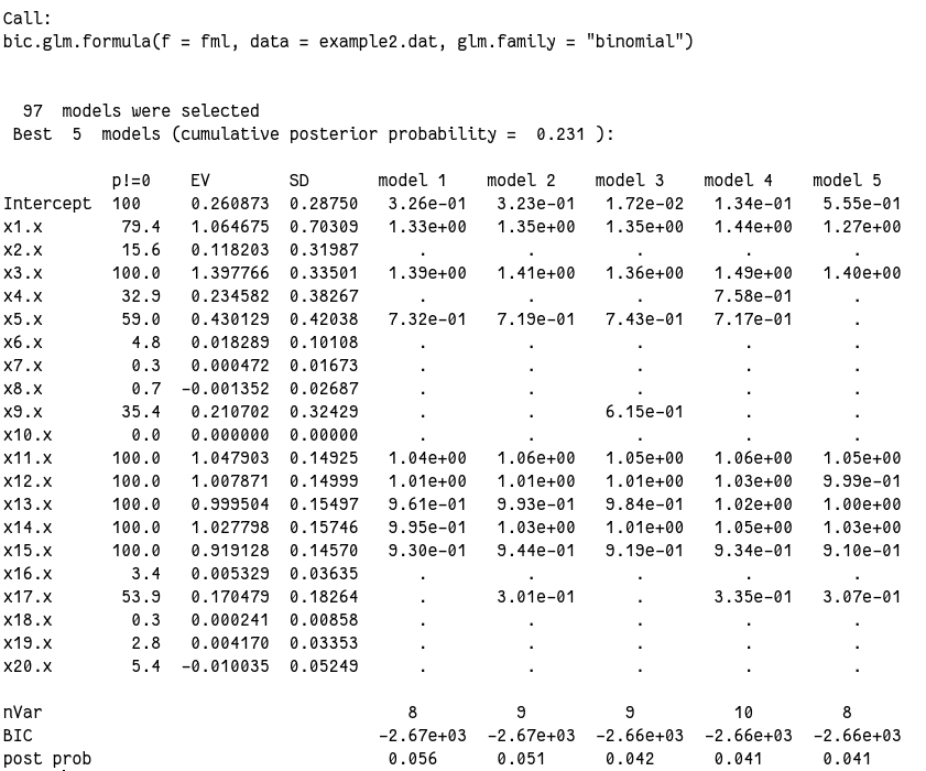
前几个模型其实都非常接近,并且和“真实”模型也很接近了。但我的结果里所有模型几乎都没有纳入 x2、x4 和 x6 ~ x10,而原文里为 x1、x3 和 x5,原文解释因为这三个变量里 1 比例太少,难以发现。但是我这个 x6 ~ x10 其实相比起来 0/1 比例很接近的,所以原因还不在这里。看均数和标准差,发现这几个变量的标准差相对均数来说都都奇大,所以算是破案了吧。今天运气不好,随机数生成的奇奇怪怪的,没办法。
另外从后验概率来看,很多变量都达到 100%,模型表现算是很出色了。而且我们还可以,连续性变量(x11~x20)变现普遍好于分类变量(x1~x10),这也是我们常说的连续性数据能包含更多的信息,把连续性数据转成分类数据损失数据信息的意思。
总的来说 BIC 模型表现还行,但是并没有找到“真实”的模型。这说明 BIC 模型有时候会偏小。
我们再来看 AIC 的表现:
 1
 2
 3
 4
 5
 6
 7
 8
 9
10
11
12
13
14
15
16
17
18
19
20
21
22
23
24
25
26
27
28
29
30
31
32
33
34
35
36
37
38
39
40
41
42
43
44
45
46
47
48
49
50
51
52
53
54
55
56
57
58
59
60
61
62
63
64
65
66
67
68
69
70
71
72
73
74
75
76
77
78
79
80
81
82
83
84
85
86
87
|
output2.aic <- glm(fml, data = example2.dat, family = "binomial")
summary(output2.aic)
#
# Call:
# glm(formula = fml, family = "binomial", data = example2.dat)
#
# Deviance Residuals:
#    Min      1Q  Median      3Q     Max
# -2.946  -0.424   0.195   0.565   2.925
#
# Coefficients:
#             Estimate Std. Error z value Pr(>|z|)
# (Intercept)  -0.5304     0.3647   -1.45   0.1459
# x1            1.4430     0.5267    2.74   0.0061 **
# x2            1.1011     0.4441    2.48   0.0132 *
# x3            1.4722     0.3474    4.24  2.3e-05 ***
# x4            0.8851     0.3432    2.58   0.0099 **
# x5            0.7944     0.2965    2.68   0.0074 **
# x6            0.3805     0.2855    1.33   0.1826
# x7            0.0703     0.2788    0.25   0.8008
# x8           -0.1907     0.2793   -0.68   0.4948
# x9            0.5860     0.2774    2.11   0.0347 *
# x10           0.1488     0.2788    0.53   0.5935
# x11           1.0633     0.1557    6.83  8.6e-12 ***
# x12           1.0856     0.1578    6.88  6.0e-12 ***
# x13           1.0724     0.1647    6.51  7.5e-11 ***
# x14           1.1253     0.1663    6.77  1.3e-11 ***
# x15           0.9311     0.1508    6.18  6.6e-10 ***
# x16           0.1707     0.1279    1.33   0.1820
# x17           0.3410     0.1319    2.59   0.0097 **
# x18           0.1079     0.1411    0.77   0.4443
# x19           0.1810     0.1414    1.28   0.2007
# x20          -0.2914     0.1429   -2.04   0.0415 *
# ---
# Signif. codes:  0 ‘***’ 0.001 ‘**’ 0.01 ‘*’ 0.05 ‘.’ 0.1 ‘ ’ 1
#
# (Dispersion parameter for binomial family taken to be 1)
#
#     Null deviance: 655.68  on 499  degrees of freedom
# Residual deviance: 354.64  on 479  degrees of freedom
# AIC: 396.6
#
# Number of Fisher Scoring iterations: 6

step.aic <- step(output2.aic)
summary(output2.aic)
#
# Call:
# glm(formula = fml, family = "binomial", data = example2.dat)
#
# Deviance Residuals:
#    Min      1Q  Median      3Q     Max
# -2.946  -0.424   0.195   0.565   2.925
#
# Coefficients:
#             Estimate Std. Error z value Pr(>|z|)
# (Intercept)  -0.5304     0.3647   -1.45   0.1459
# x1            1.4430     0.5267    2.74   0.0061 **
# x2            1.1011     0.4441    2.48   0.0132 *
# x3            1.4722     0.3474    4.24  2.3e-05 ***
# x4            0.8851     0.3432    2.58   0.0099 **
# x5            0.7944     0.2965    2.68   0.0074 **
# x6            0.3805     0.2855    1.33   0.1826
# x7            0.0703     0.2788    0.25   0.8008
# x8           -0.1907     0.2793   -0.68   0.4948
# x9            0.5860     0.2774    2.11   0.0347 *
# x10           0.1488     0.2788    0.53   0.5935
# x11           1.0633     0.1557    6.83  8.6e-12 ***
# x12           1.0856     0.1578    6.88  6.0e-12 ***
# x13           1.0724     0.1647    6.51  7.5e-11 ***
# x14           1.1253     0.1663    6.77  1.3e-11 ***
# x15           0.9311     0.1508    6.18  6.6e-10 ***
# x16           0.1707     0.1279    1.33   0.1820
# x17           0.3410     0.1319    2.59   0.0097 **
# x18           0.1079     0.1411    0.77   0.4443
# x19           0.1810     0.1414    1.28   0.2007
# x20          -0.2914     0.1429   -2.04   0.0415 *
# ---
# Signif. codes:  0 ‘***’ 0.001 ‘**’ 0.01 ‘*’ 0.05 ‘.’ 0.1 ‘ ’ 1
#
# (Dispersion parameter for binomial family taken to be 1)
#
#     Null deviance: 655.68  on 499  degrees of freedom
# Residual deviance: 354.64  on 479  degrees of freedom
# AIC: 396.6
#
# Number of Fisher Scoring iterations: 6
|
AIC 最终纳入了 13 个变量,其中 11 个变量是对的,但用纳入了两个事实上应该是无关的变量。所以 AIC 的模型倾向于偏大。
结论:AIC 和 BIC 没有二者不相伯仲,很难一句话说清楚二者谁更好。但 BIC 对于作预测表现更好,而且能鉴定混杂因素。
Example 3: Low birth weight
最后一个例子,我们使用一个真实数据来看 BIC 在模型选择上的优势。
数据是 MASS 包自带的 birthwt 数据,这是一个 189 * 10 描述低体重新生儿可能相关因素的数据:
 1
 2
 3
 4
 5
 6
 7
 8
 9
10
11
12
13
14
15
16
17
18
19
20
21
|
data("birthwt", package = 'MASS')
head(birthwt)
#    low age lwt race smoke ptl ht ui ftv  bwt
# 85   0  19 182    2     0   0  0  1   0 2523
# 86   0  33 155    3     0   0  0  0   3 2551
# 87   0  20 105    1     1   0  0  0   1 2557
# 88   0  21 108    1     1   0  0  1   2 2594
# 89   0  18 107    1     1   0  0  1   0 2600
# 91   0  21 124    3     0   0  0  0   0 2622
str(birthwt)
# 'data.frame':	189 obs. of  10 variables:
#  $ low  : int  0 0 0 0 0 0 0 0 0 0 ...
#  $ age  : int  19 33 20 21 18 21 22 17 29 26 ...
#  $ lwt  : int  182 155 105 108 107 124 118 103 123 113 ...
#  $ race : int  2 3 1 1 1 3 1 3 1 1 ...
#  $ smoke: int  0 0 1 1 1 0 0 0 1 1 ...
#  $ ptl  : int  0 0 0 0 0 0 0 0 0 0 ...
#  $ ht   : int  0 0 0 0 0 0 0 0 0 0 ...
#  $ ui   : int  1 0 0 1 1 0 0 0 0 0 ...
#  $ ftv  : int  0 3 1 2 0 0 1 1 1 0 ...
#  $ bwt  : int  2523 2551 2557 2594 2600 2622 2637 2637 2663 2665 ...
|
具体变量的意思可以 ??birthwt 查看,我这里截图的原文里的:
我们把分类变量转变成 factor,并且由于是做 Logistic 回归所以 bwt 这一列也不要了:
 1
 2
 3
 4
 5
 6
 7
 8
 9
10
11
12
13
14
15
16
17
18
19
20
21
22
|
birthwt$smoke <- as.factor(birthwt$smoke)
birthwt$race <- as.factor(birthwt$race)
birthwt$ptl <- as.factor(birthwt$ptl)
birthwt$ht <- as.factor(birthwt$ht)
birthwt$ui <- as.factor(birthwt$ui)

birthwt <- subset(birthwt, select = -c(id, bwt))
summary(birthwt)
 #      low             age            lwt      race   smoke   ptl     ht
 # Min.   :0.000   Min.   :14.0   Min.   : 80   1:96   0:115   0:159   0:177
 # 1st Qu.:0.000   1st Qu.:19.0   1st Qu.:110   2:26   1: 74   1: 24   1: 12
 # Median :0.000   Median :23.0   Median :121   3:67           2:  5
 # Mean   :0.312   Mean   :23.2   Mean   :130                  3:  1
 # 3rd Qu.:1.000   3rd Qu.:26.0   3rd Qu.:140
 # Max.   :1.000   Max.   :45.0   Max.   :250
 # ui           ftv
 # 0:161   Min.   :0.000
 # 1: 28   1st Qu.:0.000
 #         Median :0.000
 #         Mean   :0.794
 #         3rd Qu.:1.000
 #         Max.   :6.000
|
然后就可以了:
1
2
3
|
output2 <- bic.glm(low ~ age + lwt + smoke + ptl + ht + ui +
                       ftv + race, glm.family = binomial, data = birthwt)
summary(output2)
|
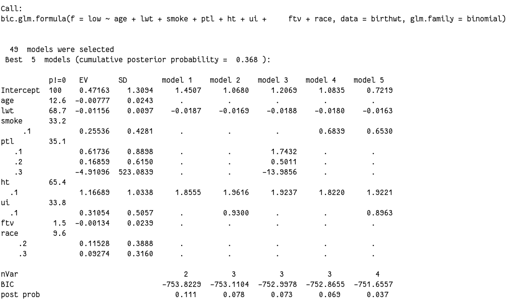
看看其他的:
 1
 2
 3
 4
 5
 6
 7
 8
 9
10
11
12
13
14
15
16
|
output3$postprob
#  [1] 0.110709 0.077529 0.073286 0.068595 0.037462 0.034935 0.033014 0.026886 0.026275 0.025975 0.024136 0.023395
# [13] 0.022719 0.022593 0.022368 0.022217 0.020016 0.018094 0.015331 0.015111 0.014675 0.014476 0.014436 0.014214
# [25] 0.013791 0.013338 0.013117 0.012539 0.011803 0.011757 0.010826 0.010659 0.008751 0.008403 0.008373 0.008184
# [37] 0.008096 0.007983 0.007936 0.007680 0.007018 0.006979 0.006709 0.006611 0.006575 0.006431 0.006249 0.006180
# [49] 0.005564
output3$names
# [1] "age"   "lwt"   "smoke" "ptl"   "ht"    "ui"    "ftv"   "race"
output3$probne0
#   age   lwt smoke   ptl    ht    ui   ftv  race
#  12.6  68.7  33.2  35.1  65.4  33.8   1.5   9.6
output3$postmean
# (Intercept)         age         lwt      smoke1        ptl1        ptl2        ptl3         ht1         ui1
#    0.471634   -0.007765   -0.011558    0.255357    0.617360    0.168588   -4.910963    1.166893    0.310537
#         ftv       race2       race3
#   -0.001339    0.115279    0.092740
|
在模型中比例最高的 lwt 也只有 68%,所以总体来说都所以变量证据都不够。
总结
实际运用最好还是 AIC 和 BIC 都考虑一下,然后还要结合专业知识实际考虑变量的纳入和剔除。如果有足够的专业只是认为一个变量无论计算结果如何,都应该纳入模型,那么这时候当然应该纳入。BIC 里使用 set.prior = 1 就行了。
同时,如果模型的目的是做预测,那么其实应该哪些变量纳入并不重要,只要模型拟合的足够好就行了。但是如果是为了看哪些因素比较重要以及各变量和结果之间的关系强弱,这时候才必须要考虑这个问题。
code: logselect.BMA.R